library(lares)
library(tidyverse)
library(tidymodels)
library(themis)
library(tidyposterior)
library(SmartEDA)
library(DataExplorer)
library(skimr)
library(ggpubr)
library(workflowsets)Penanganan Class Imbalanced pada KNN dengan tidymodels
R Programming
Statistical Machine Learning
tidymodels
Package
Deskripsi singkat data
Tutorial kali ini akan menggunakan data yaitu German df. Berikut adalah informasi singkat mengenai data
This dataset classifies people described by a set of attributes as good or bad df risks.
Author: Dr. Hans Hofmann Source: UCI - 1994 Please cite: Dua, D. and Graff, C. (2019). UCI Machine Learning Repository [http://archive.ics.uci.edu/ml]. Irvine, CA: University of California, School of Information and Computer Science.
Attribute description
- Status of existing checking account, in Deutsche Mark.
- df history (dfs taken, paid back duly, delays, critical accounts)
- Purpose of the df (car, television,…)
- df amount
- Status of savings account/bonds, in Deutsche Mark.
- Present employment, in number of years.
- Installment rate in percentage of disposable income
- Personal status (married, single,…) and sex
- Other debtors / guarantors
- Present residence since X years
- Property (e.g. real estate)
- Age in years
- Other installment plans (banks, stores)
- Housing (rent, own,…)
- Number of existing dfs at this bank
- Job
- Number of people being liable to provide maintenance for
- Telephone (yes,no)
- Foreign worker (yes,no)
- Duration in months
data ini bisa diperoleh di link berikut ini
Import data di R
df <- read_csv("german_credit.csv") %>%
      # convert all character column to factor
      mutate(across(where(is.character),as.factor))
Rows: 1000 Columns: 21
── Column specification ────────────────────────────────────────────────────────
Delimiter: ","
chr (14): checking_status, credit_history, purpose, savings_status, employme...
dbl (7): duration, credit_amount, installment_commitment, residence_since, ...
ℹ Use `spec()` to retrieve the full column specification for this data.
ℹ Specify the column types or set `show_col_types = FALSE` to quiet this message.glimpse(df)Rows: 1,000
Columns: 21
$ checking_status <fct> '<0', '0<=X<200', 'no checking', '<0', '<0', 'n…
$ duration <dbl> 6, 48, 12, 42, 24, 36, 24, 36, 12, 30, 12, 48, …
$ credit_history <fct> 'critical/other existing credit', 'existing pai…
$ purpose <fct> radio/tv, radio/tv, education, furniture/equipm…
$ credit_amount <dbl> 1169, 5951, 2096, 7882, 4870, 9055, 2835, 6948,…
$ savings_status <fct> 'no known savings', '<100', '<100', '<100', '<1…
$ employment <fct> '>=7', '1<=X<4', '4<=X<7', '4<=X<7', '1<=X<4', …
$ installment_commitment <dbl> 4, 2, 2, 2, 3, 2, 3, 2, 2, 4, 3, 3, 1, 4, 2, 4,…
$ personal_status <fct> 'male single', 'female div/dep/mar', 'male sing…
$ other_parties <fct> none, none, none, guarantor, none, none, none, …
$ residence_since <dbl> 4, 2, 3, 4, 4, 4, 4, 2, 4, 2, 1, 4, 1, 4, 4, 2,…
$ property_magnitude <fct> 'real estate', 'real estate', 'real estate', 'l…
$ age <dbl> 67, 22, 49, 45, 53, 35, 53, 35, 61, 28, 25, 24,…
$ other_payment_plans <fct> none, none, none, none, none, none, none, none,…
$ housing <fct> own, own, own, 'for free', 'for free', 'for fre…
$ existing_credits <dbl> 2, 1, 1, 1, 2, 1, 1, 1, 1, 2, 1, 1, 1, 2, 1, 1,…
$ job <fct> skilled, skilled, 'unskilled resident', skilled…
$ num_dependents <dbl> 1, 1, 2, 2, 2, 2, 1, 1, 1, 1, 1, 1, 1, 1, 1, 1,…
$ own_telephone <fct> yes, none, none, none, none, yes, none, yes, no…
$ foreign_worker <fct> yes, yes, yes, yes, yes, yes, yes, yes, yes, ye…
$ class <fct> good, bad, good, good, bad, good, good, good, g…Penanganan Imbalanced Data
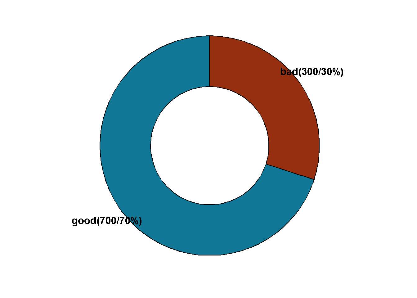
df %>%
  count(class) %>%
  rename(cat=class) %>%
  mutate(label=str_c(cat,"(",n,"/",
                     round(n*100/sum(n),2),"%)")
         ) %>%
  ggdonutchart(x="n",label = "label",
               fill = c("#962E10","#107896"),
               lab.pos = "out",
               lab.font = c(5,"bold","black")
               )
Random Over sampling (ROS)
upsm_try <- map(seq(0.5,1.25,0.25),function(x) {
recipe(class~.,data = df) %>%
step_upsample(class,over_ratio = x,skip = FALSE) %>%
    prep() %>%
    bake(new_data = df) %>%
    count(class,name = str_c("Oversampling ",x))
})
upsm_try
[[1]]
# A tibble: 2 × 2
class `Oversampling 0.5`
<fct> <int>
1 bad 350
2 good 700
[[2]]
# A tibble: 2 × 2
class `Oversampling 0.75`
<fct> <int>
1 bad 525
2 good 700
[[3]]
# A tibble: 2 × 2
class `Oversampling 1`
<fct> <int>
1 bad 700
2 good 700
[[4]]
# A tibble: 2 × 2
class `Oversampling 1.25`
<fct> <int>
1 bad 875
2 good 875Output diatas adalah efek pemilihan over_ratio terhadap pertambahan class minority bad. Selanjutnya kita pilih over_ratio=1
upsm <- recipe(class~.,data = df) %>%
        step_upsample(class,over_ratio = 1)
Random Under sampling (RUS)
undersm_try <- map(seq(0.5,1.25,0.25),function(x) {
recipe(class~.,data = df) %>%
step_downsample(class,under_ratio = x,skip = FALSE) %>%
    prep() %>%
    bake(new_data = df) %>%
    count(class,name = str_c("Undersampling ",x))
})
undersm_try
[[1]]
# A tibble: 2 × 2
class `Undersampling 0.5`
<fct> <int>
1 bad 150
2 good 150
[[2]]
# A tibble: 2 × 2
class `Undersampling 0.75`
<fct> <int>
1 bad 225
2 good 225
[[3]]
# A tibble: 2 × 2
class `Undersampling 1`
<fct> <int>
1 bad 300
2 good 300
[[4]]
# A tibble: 2 × 2
class `Undersampling 1.25`
<fct> <int>
1 bad 300
2 good 375Output diatas adalah efek pemilihan under_ratio terhadap pengurangan class majority good. Selanjutnya kita pilih under_ratio=1
undersm <- recipe(class~.,data = df) %>%
            step_downsample(class,under_ratio = 1)
Synthetic Minority Over-sampling Technique (SMOTE)
Penerapan metode SMOTE hanya bisa dilakukan untuk peubah prediktor numerik. Jika terdapat peubah prediktor kategorik seperti pada data ini, maka terdapat dua solusi yang mungkin yaitu:
- Menggunakan metode SMOTE-NC (baca jurnal di link berikut) yang bisa diterapkan di peubah prediktor kategorik maupun peubah prediktor numerik. Namun, SMOTE-NC belum tersedia di ekosistem
mlr3(November 2021). - Melakukan Categorical Variable Encoding, yaitu transformasi peubah prediktor kategorik ke peubah prediktor numerik. Metode-metode apa saja yang termasuk Categorical Variable Encoding bisa dilihat pada link berikut ini
Fungsi step_smote dari package themis menggunakan metode SMOTE yang hanya bisa diterapkan pada prediktor numerik saja
smote_try <- try(map(seq(0.5,1.25,0.25),function(x) {
recipe(class~.,data = df) %>%
step_smote(class,over_ratio = x,skip = FALSE) %>%
    prep() %>%
    bake(new_data = df) %>%
    count(class,name = str_c("Undersampling ",x))
}))
Error in map(seq(0.5, 1.25, 0.25), function(x) { : ℹ In index: 1.
Caused by error in `step_smote()`:
Caused by error in `prep()`:
✖ All columns selected for the step should be double or integer.
• 13 factor variables found: `checking_status`, `credit_history`, …Sementara itu jika prediktor yang dimiliki terdapat prediktor numerik dan prediktor kategorik bisa menggunakan fungsi step_smotenc dari package themis
smote_try <- map(seq(0.5,1.25,0.25),function(x) {
recipe(class~.,data = df) %>%
step_smotenc(class,over_ratio = x,skip = FALSE) %>%
    prep() %>%
    bake(new_data = df) %>%
    count(class,name = str_c("Undersampling ",x))
})
smote_try
[[1]]
# A tibble: 2 × 2
class `Undersampling 0.5`
<fct> <int>
1 bad 350
2 good 700
[[2]]
# A tibble: 2 × 2
class `Undersampling 0.75`
<fct> <int>
1 bad 525
2 good 700
[[3]]
# A tibble: 2 × 2
class `Undersampling 1`
<fct> <int>
1 bad 700
2 good 700
[[4]]
# A tibble: 2 × 2
class `Undersampling 1.25`
<fct> <int>
1 bad 875
2 good 875Output diatas adalah efek pemilihan over_ratio terhadap pertambahan class minority bad. Selanjutnya kita pilih over_ratio=1
smote_fin <- recipe(class~.,data = df) %>%
             step_smotenc(class,over_ratio = 1)
Pemodelan KNN
Menyiapkan Pembagian Data
K-fold Cross Validation
set.seed(345)
folds <- vfold_cv(df, v = 10,strata = "class")
Contoh visualisasi 100 amatan pertama di setiap folds
tidy(folds) %>%
  filter(Row<101) %>%
ggplot(aes(x = Fold, y = Row,fill = Data)) +
    geom_tile()+
  theme_lares()
Warning in .font_global(font, quiet = FALSE, ...): Font(s) "Arial Narrow" not
installed, with other name, or can't be found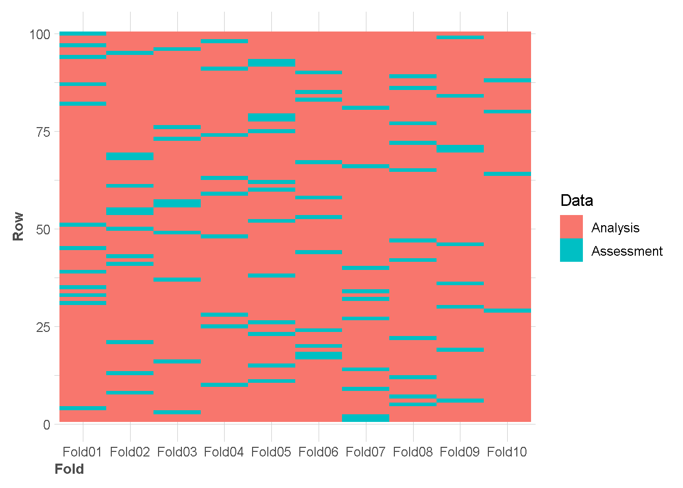
Mendefinisikan Model KNN
knn_tune <- nearest_neighbor(neighbors=tune(),
                        weight_func="rectangular") %>%
  set_engine("kknn") %>%
  set_mode("classification")
knn_grid <- grid_regular(neighbors(range = c(2,50)),
levels= 50)
knn_grid Komparasi, Tuning dan Evaluasi Model
Menkombinasikan metode class imbalanced dan model
models <- list(knn=knn_tune)
preproc <- list(over_sample=upsm,
                under_sample=undersm,
                smote=smote_fin)
wf_set <- workflow_set(preproc = preproc,models = models)
Running models
models_eval <- workflow_map(wf_set,
                            fn="tune_grid",
                            resamples = folds,
                            control=control_grid(save_workflow = TRUE),
                            metrics=metric_set(accuracy,
                                               bal_accuracy),
                            grid = knn_grid,
                            seed = 2123)
Evaluasi model
## custom function
extract_neighbor <- function(wflw_res) {
  map(seq_along(wflw_res$wflow_id), function(i) {
    id <- wflw_res$wflow_id[i]
    res <- extract_workflow_set_result(wflw_res, id = id) %>%
      collect_metrics() %>%
      mutate(wflow_id = id,
             .config = NULL,
             .estimator = NULL) %>%
      relocate(wflow_id)
    return(res)
  }) %>%
    list_rbind()
}
## custom function
plot_neighbor<- function(knn_result,metric){
knn_result %>%
filter(.metric%in%metric) %>%
mutate(wflow_id=str_remove_all(wflow_id,"_knn")) %>%
ggplot(aes(x=neighbors, y=mean,col=wflow_id)) +
geom_line()+
geom_point()+
ylab(metric) +
scale_x_continuous(n.breaks = 12)+
theme_lares()+
theme(legend.position = "top")
}## metric used information
metric_used <- models_eval %>%
collect_metrics() %>%
pull(.metric) %>%
unique()
metric_used[1] "accuracy" "bal_accuracy"neighbors_result <- extract_neighbor(models_eval)
neighbors_result %>%
plot_neighbor(metric = metric_used[1])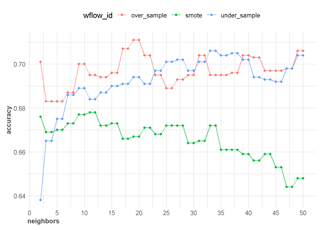
neighbors_result %>%
    plot_neighbor(metric = metric_used[2])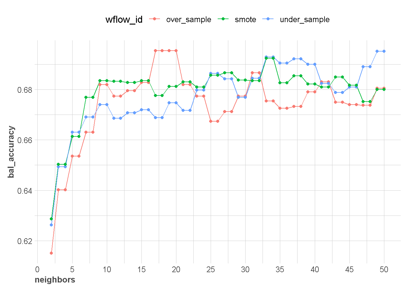
Menentukan Model terbaik dan Training
mod_best1 <- fit_best(x = models_eval,metric = "accuracy")
mod_best1
══ Workflow [trained] ══════════════════════════════════════════════════════════
Preprocessor: Recipe
Model: nearest_neighbor()
── Preprocessor ────────────────────────────────────────────────────────────────
1 Recipe Step
• step_upsample()
── Model ───────────────────────────────────────────────────────────────────────
Call:
kknn::train.kknn(formula = ..y ~ ., data = data, ks = min_rows(19L, data, 5), kernel = ~"rectangular")
Type of response variable: nominal
Minimal misclassification: 0.2628571
Best kernel: rectangular
Best k: 19mod_best2 <- fit_best(x = models_eval,metric = "bal_accuracy")
mod_best2══ Workflow [trained] ══════════════════════════════════════════════════════════
Preprocessor: Recipe
Model: nearest_neighbor()
── Preprocessor ────────────────────────────────────────────────────────────────
1 Recipe Step
• step_upsample()
── Model ───────────────────────────────────────────────────────────────────────
Call:
kknn::train.kknn(formula = ..y ~ ., data = data, ks = min_rows(17L, data, 5), kernel = ~"rectangular")
Type of response variable: nominal
Minimal misclassification: 0.2578571
Best kernel: rectangular
Best k: 17Prediksi Data baru
Berikut kita generate data baru dummy
set.seed(1234)
data_baru <- df %>%
              slice_sample(n = 2,by = class) %>%
              select(-class)
data_baru
pred_data_baru2 <- mod_best1 %>%
predict(new_data = data_baru)
pred_data_baru3 <- mod_best2 %>%
predict(new_data = data_baru)pred_data_baru2pred_data_baru3